Estimating the speed of an algorithm
One really useful thing to be able to do when discussing algorithms is to say how fast they are. The most direct way to find out how fast an algorithm is, is to code it up and run it. One big problem with this approach is that coding up an algorithm is time consuming -- especially if you include debugging time. In a competition like the AIO where you have limited time, you really want to know if your algorithm is going to run in time before you start coding it up. Is there a good way to estimate this? We use time complexity analysis and big O notation to reason about algorithm speed.
Before we discuss these two topics, let's take a short detour to explain some of the intuition behind big O notation and complexity analysis.
Counting triplets
Let's consider a simple problem: How many ways can you write a number \(N\) as the sum of three distinct positive numbers? For example \(2 + 3 + 5\), \(5 + 2 + 3\) and \(7 + 1 + 2\) are all ways that we can write \(10\). \(0 + 4 + 6\) and \(3 + 3 + 4\) are not valid. You might have some ideas already about how to do this, but let's consider the following two algorithms (given in psuedocode):
| Algo 1 | Algo 2 |
|---|---|
|
|
Examining the two algorithms above, it's not too hard to see that Algo 2 is doing something cleverer than Algo 1, and will be faster.
To really see the difference in speed, I've implemented both algorithms and tabulated their run times for various values of \(N\):
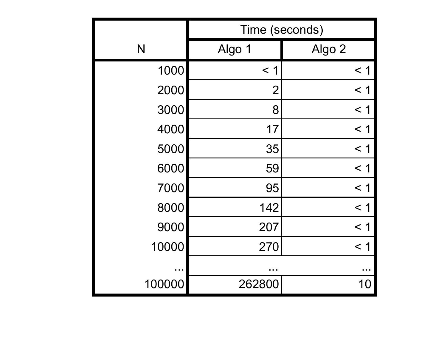
When \(N\) is 1000, both run very quickly, less than a second. However as \(N\) becomes larger and larger, the slowness of Algo 1 begins to show. It takes nearly ~5 minutes to run for \(N = 10\,000)\), while Algo 2 is still really fast. The difference becomes even more pronounced for \(N = 100\,000\): Algo 1 took about 3 days to complete, while Algo 2 took ~10 seconds.
Although our empirical experiment shows Algo 1 to be unsalvageably slow compared to Algo 2, perhaps there is hope yet to improve it, to a point where it is comparable?
# While searching for triplets, we will iterate so that i < j < k.
# This will cut down on the number of triplets we have to search.
# At the end, we multiply the count by 6, since each triplet we found can be arranged in six different ways.
# e.g. For N = 10 and the triplet 2, 3 and 5:
# 2 + 3 + 5 = 10
# 2 + 5 + 3 = 10
# 3 + 2 + 5 = 10
# 3 + 5 + 2 = 10
# 5 + 3 + 2 = 10
# 5 + 2 + 3 = 10
count = 0
for i = 1 to N:
    for j = i+1 to N:
        for k = j+1 to N:
            if i, j and k sum to N:
                count += 1

output count*6
Don't worry too much about understanding the psuedocode. The important part is, this optimization cuts down the number of iterations to about \(N^3/6\). From here, we could optimize the code even more:
count = 0
# i can't be more than N/3. If it were, then j > N/3 and k > N/3, so i + j + k would be more than N
for i = 1 to N/3:
    # We can similarly reason that j can't be more than (N-1)/2
    for j = i+1 to (N-i)/2:
        for k = j+1 to N:
            if i, j and k sum to N:
                count += 1

output count*6
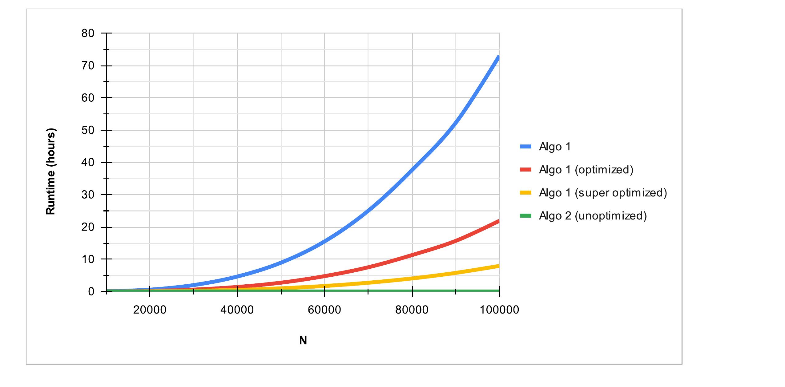
These super-optimized variations of Algo 1 do run considerably faster, but you can still see that they do not even come close to Algo 2's run time. For \(N = 100\,000\), the super-optmized algorithm still takes about 8 hours.
One way to think of this is that an algorithm doing \(N^3\) steps is fundamentally worse than an algorithm that does \(N^2\) in a way that no amount of optimization can hope to fix. If we plot the runtimes of Algo 1 and its optmized variants alongside Algo 2, we can see just how drastic the difference is.
Big O Notation
We use big O notation to describe the speed of an algorithm. Big O notation tells us how one quantity (e.g. an algorithm's running time) grows as another quantity (e.g. the size of the input) grows. It is not very precise (you could never calculate the running time of a program just by knowing its time complexity), but it is usually easy to calculate and it gives us most of the information we need. For example, let's say we have a list of \(N\) numbers:
- "The number of names on the list" is n. We say this value is \(O(N)\), pronounced "order n". We also say that this value is linear.
- “The number of names in the first half of the list” is \(N/2\). We also say that this value is \(O(N)\), because we are not interested in multiplication or division by constant factors. (For example, \(144N\) would also be considered \(O(N)\).)
- "The number of squares in an N by N grid" is \(N^2\) . We say that this value is \(O(N^2)\), or quadratic.
- "The number of ways of choosing one person from the first half of the list, and one person from the second half" is \((N/2)(N/2) = N^2/4\). We say that this value is \(O(N^2)\).
- "The number of ways of choosing a leader and a deputy leader from the list" is \(N(N - 1) = N^2 - N\). (There are \(N\) people who we can choose to be leader, and then \(N - 1\) remaining people who we can choose to be deputy leader). We ignore the \(N\) in \(N^2 - N\) and say the value is \(O(N^2)\) because in some sense it is ‘smaller’ than the \(N^2\)).
- "The number of letters in the English alphabet" is 26. It has nothing to do with \(N\), and we say that this value is \(O(1)\), or constant.
- "The number of times you can halve the list before only one name is left" is approximately \(\log_2N\). The ‘change of base rule’ tells us that logarithms with different bases are multiples of each other, and so we omit the base and say this value is \(O(\log N)\), or logarithmic. (If you’re not familiar with logarithms, just ignore this for now).
- "The number of ways of choosing three different people from the list" is \(\frac{N(N-1)(N-2)}{3 \times 2 \times 1} = \frac{1}{6}(N^3 - 3N^2 + 2N)\). (Convince yourself of this). We ignore the \(\frac{1}{6}\) as we are not interested in constant factors. We ignore the \(3N^2\) and the \(2N\) because in some sense they are 'smaller' than \(N^3\). We say that this value is \(O(N^3)\), or cubic.
What do we mean when we say that \(3N^2\) is 'smaller' than \(N^3\)? Surely this isn't true for all \(N\) (e.g. when \(N = 2\), \(3N^2 = 12 \nless N^3 = 8\)).
In this case, as soon as \(N > 3\), then \(N^3\) becomes bigger than \(3N^2\), and remains bigger no matter how large \(N\) gets. We can graph the two functions and see just how dramatic the difference becomes.
What's more, this fact remains even if we were to replace 3 with some other number. Any multiple of \(N^2\) will eventually be outpaced by the growth \(N^3\). Even \(100N^2\) is eventually outpaced by \(N^3\). It is this kind of long-term behaviour that big O notation is used to describe. The major big O classes we are concerned with are:
\(O(1) < O(\log N) < O(N) < O(N \log N) < O(N^2) < O(N^3) < \ldots < O(2^N) < O(3^N) < \ldots\)
Time Complexity
We often talk about the time complexity of an algorithm. The is just big O notation being used to describe how long the program runs (roughly), depending on the input size. However we have to be slightly more specific than this. How fast an algorithm is depends not only on the input size, but on other properties of the input as well.
For example, consider the following C++ code to search an array with \(K\) elements for the value \(x\). (We assume that the array does contain \(x\)).
for (int i = 0; i < K; i++) {
    if (v[i] == x) {
        return i;
    }
}
The return statement ends the loop as soon as it is run. This means that the program takes different amounts of time depending on where \(x\) is in the list.
For a simple program such as this, we can even calculate the exact number of C++ instructions the program takes (counting the instructions as i = 0, i < K, i++, v[i] == x, return i). If \(x\) is at position \(j\) in the array, then the program will run for \(3j + 1\) instructions.
Now, consider how big O notation can be used to analyse this:
-
In the very best case, the first value in the array (v[0]) is \(x\). The code inside the loop is only run once, no matter how big \(K\) is. Approximately 4 instructions are run.
We say the best case time complexity of this algorithm is \(O(1)\). We also say it runs in best-case constant time.
-
On average (assuming \(x\) could be anywhere in the list), \(x\) turns up halfway through the list. Approximately \(3(\frac{K}{2}) + 1\) instructions are run.
We say the average case time complexity of this algorithm is \(O(K)\). We also say it runs in average-case linear time.
-
In the very worst case, \(x\) is at the end of the array (v[K-1]). Approximately \(3K + 1\) instructions are run.
We say the worst case time complexity of this algorithm is \(O(K)\). We also say it runs in worst-case linear time.
Usually when people are talking about the time complexity of an algorithm, they are talking about this last one.
To calculate these time complexities, we used a formula that counted the exact number of lines of code executed. But what about different programming languages, where loops might be written differently? What if we tried replacing the i < K inside the loop with v[i] != x, to save on instructions? What would the formula look like then? What about other problems?
In fact, it doesn't matter! Although these changes and tweaks will have an effect on the number of lines of code that are run, they will not change the time complexity, which remains \(O(K)\). You can only change the time complexity by using a different algorithm altogether.
The time complexity of an algorithm is independent of its implementation. It has nothing to do with what language it is written in, how many extra variables are used, or how many lines of code any particular step takes. In fact, we can tell the time complexity of an algorithm without needing to look at actual code. For example, the previous algorithm might be phrased as:
For each value in the array
    If that value is equal to x, return its position
Say this array contains \(K\) elements. Checking if a value is equal to \(x\) is 'quick' (constant time). In the worst case we need to check all K values. From this, we can immediately say that the worst case time complexity of the algorithm is \(O(K)\).
Our use of big O ntoation allows us to avoid micro-optimization (tweaking an implementation for a small increase in speed) and concentrate on macro-optimization (modifying the algorithm to improve the big O time complexity, resulting in a dramatic increase in speed).
We are most interested in the worst-case running time of algorithms. This is usually what we refer to when we say, 'The time complexity of algorithm X is...'. One reason for this is that if we know that our program is 'fast enough' (i.e. under the time limit) in the worst case, then we know it will be fast enough in any case. This means we only ever need to worry about this measure of speed.
In the AIO and other informatics competitions, your submitted code will almost certainly be subjected to worst case inputs. The test data pushes programs to the limits in order to reward students who implement faster algorithms (ones with lower time complexity).