Problem 6 - Atlantis III: Twin Rivers

Here, we will discuss the solution to Atlantis III: Twin Rivers from AIO 2024.

This is a very difficult problem designed to challenge the very top students in Australia, so do not worry if you are struggling to understand the solution!

Solution

Subtask 1: N, T, L ≤ 2000, R_i = 1 for all i and S_j = 2 for all j. That is, all existing bridges cross the 1st river and every trip finishes on Strip 2.

In this subtask, bridges and trips only cross the first river.

Before considering where to place the new bridge, let's first consider how to calculate the length of a trip. Clearly we need to walk along Strip 1 (possibly walking 0 distance if there is a bridge at our starting point), cross a bridge to Strip 2, and then walk to our destination. If we play around with some examples on pen and paper, it should become clear that it is always fastest to cross only one bridge as opposed to crossing back and forth.

After seeing this it should become clear that the fastest path is to travel to the closest bridge to our starting location, cross it, and then travel to the destination. If the distance to the closest bridge is d then the total distance of this trip will be 2d + 1.

Let's try and use this to solve the first subtask with a brute force algorithm.

Clearly our new bridge should cross the first river and so there are L+1 possible locations to consider, from 0 to L kilometers from the left of the city. For each of these, we can try to calculate the cost of each of the T trips by finding the closest bridge. The simplest way to do this would be to loop over all the N existing bridges as well as the new bridge to see which is closest to the trip's X coordinate. After calculating the cost of every trip, we can sum these to get the sum of distances for a particular new bridge location. We can then take the minimum sum over all the possible new bridge locations to get our final answer.

How long does this algorithm take? We loop over L+1 possible bridge locations, and for each of those we loop over T trips, and for each of those we consider N+1 bridges so our overall time complexity is O(LTN). Unfortunately, this is a bit too slow given our bounds of N, T, L ≤ 2000. (2000³ = 8 billion, while we usually want to aim for something around 100 million operations in a second to be safely within the time limit.)

How can we speed up this algorithm?

One way is to precompute the current closest bridge for each trip before adding the new bridge, and then for each new bridge location and for each trip, we can check whether the new bridge is closer than the current closest bridge. This lets us skip looping over all N existing bridges for every trip.

We can find the current closest bridge for each trip by simply looping over all bridges for each trip, taking O(TN) time. Then, to find the answer we can loop over all L+1 possible new bridge locations as before. And for each of them, we can loop over all T trips and to find the new length of this trip we only need to compare the current closest bridge with the new bridge, which takes a constant amount of time. So this part of the algorithm now takes O(LT) time instead of O(LTN) time.

Thus our overall time complexity becomes O(TN + LT) = O(T(N+L)) time which is fast enough to solve subtask 1. (T(N+L) = 2000 × (2000 + 2000) = 8 million, so our algorithm should run well within the time limit.)

Subtask 2: R_i = 1 for all i and S_j = 2 for all j. That is, all existing bridges cross the 1st river and every trip finishes on Strip 2.

In subtask 2, all bridges and trips cross only the first river just like subtask 1, but there are no special restrictions on the length of the city or the number of bridges or trips anymore. Thus our algorithm for subtask 1 will be too slow.

How can we speed up our algorithm even further?

Let's consider a single trip and think about how the new bridge affects the length of this trip. If we play around on pen and paper we can make the following observation:

Observation: For a given trip with coordinate X, let the current distance to the closest bridge be d (so the current trip distance is 2d + 1).

• If the new bridge is at X-d or to the left then the trip distance is unchanged.
• Otherwise, as the new bridge moves right 1km at a time from X-d to X, the trip distance decreases by 2km each step.
• Then, as the new bridge moves right 1km at a time from X to X+d, the trip distance increases back up by 2km each step.
• Finally, if the new bridge is at X+d or to the right, the trip distance is the same as the original distance.

We can see why this should be the case. If the new bridge is further than the current closest bridge, then the trip distance will be unchanged because we will just take the current closest bridge and ignore the new one. Otherwise, each kilometer that the new bridge is closer will save us 2km in travel time, 1km going to the bridge and 1km coming back from it to our destination.

Using this observation, we can see that as we move our new bridge from left to right, the length of a particular trip will have 4 'stages': a stage where the distance of the trip is constant, a decreasing distance stage, an increasing distance stage, and finally another constant stage.

We can use this to speed up our algorithm as follows: Instead of calculating the length of every trip for every new bridge location, we will instead calculate the length of every trip once and then keep track of how the trip lengths change as we move the new bridge from left to right. Here is some pseudocode illustrating this idea:

• Pseudocode

let sum = sum of starting lengths of all trips
let answer = sum
let rate_of_change = 0
let updates[] be an array storing changes to the rate_of_change

# calculate updates[]
for each trip i (with coordinate X[i]),
    find d = current distance to closest bridge
    updates[X-d] -= 2
    updates[X] += 4       # +4 to go from -2km each step to +2km each step
    updates[X+d] -= 2     # -2 to go from +2km each step to +0km each step

for each position bridge position i from -L to 2*L,
    sum += rate_of_change
    answer = min(answer, sum)
    rate_of_change += updates[i]

Note that in this pseudocode we loop from -L to 2L because the points X-d and X+d could be outside the range [0, L]. To actually implement this you could increase all coordinates by L to make all array indices positive, or you could modify the code to start the calculation at bridge position 0.

This algorithm takes O(L+T) time, the speed up comes from the fact that we only need to do a constant amount of work for each trip instead of having to recalculate the cost of each trip for every possible new bridge position. This kind of technique where we sweep through all possible answers and keep track of the current cost is sometimes called a 'sweep line' or 'sweep' algorithm.

We also need to precalculate the closest bridge to each trip faster than in subtask 1. Since the bridge locations are given in sorted order, we can do this in O(N+T) time. Our final time complexity is O(L+T+N).

Subtask 3: R_i = 1 for all i and S_j = 3 for all j. That is, all existing bridges cross the 1st river and every trip finishes on Strip 3.

In this subtask, we introduce trips across both rivers. In fact, every trip crosses both rivers, and since all existing bridges cross the first river, we must place our new bridge across the second river.

Again, let's start by figuring out how to find the shortest path for a given trip across both rivers if we have a fixed set of bridges (including bridges across both rivers). Firstly, we can see that it is always optimal to take exactly two bridges rather than travel back and forth between strips. Drawing out some cases, we can also observe the following:

Observation: Given a trip starting at coordinate X on Strip 1, it is always optimal to cross river 1 at either:

• the closest bridge to the left of X if one exists (bridge coordinate ≤ X), or
• the closest bridge to the right of X if one exists (bridge coordinate ≥ X)

Proof: Suppose an optimal path uses a different bridge to cross river 1. Let's say this bridge is to the left of X (if it's to the right we can use a similar argument but on the other side). Say this bridge has x-coordinate X_O (O for optimal) and the closest bridge to the left has coordinate X_L. So we have X_O < X_L ≤ X.

The optimal path walks along Strip 1 and then crosses at X_O. But we can replace this part with a path that walks along Strip 1 from X to X_L, crosses the bridge at X_L then walks along Strip 2 to X_O. Since X_L is between X_O and X this path has the same length and therefore must also be optimal. QED

Based on this observation, we can see that the length of a trip will be the minimum of the path length going through the closest bridge to the left and the path length going through the closest bridge to the right. We could use this to implement a brute force solution for this subtask where we loop through every possible new bridge location, then calculate the sum of trip lengths by looping through every trip and taking the minimum of these two values. This solution would have time complexity O(LT + N) (+ N to precalculate the closest bridge to the left and right for each trip), which is unfortunately too slow.

Improving the time complexity

To improve the time complexity we can do something similar to subtask 2.

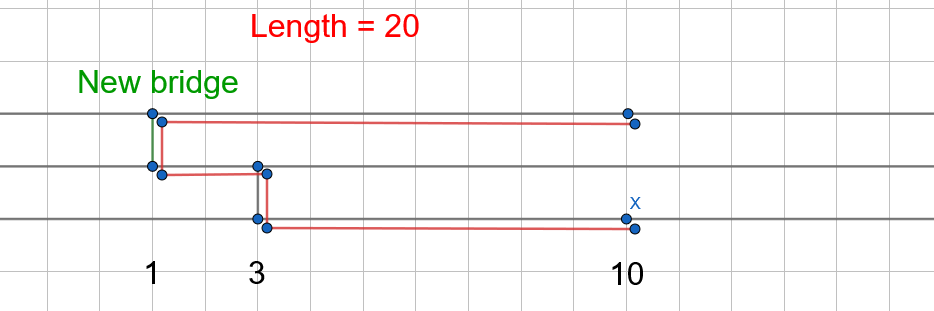
Let's consider only one of the 'closest' bridges across river 1, say the closest bridge to the left of X. Remember, the new bridge must be across river 2. Let's consider how the trip length changes as we move the new bridge from left to right across river 2.

• Initially the new bridge starts out all the way to the left, and the optimal path is to move left, cross river 1, move even further left, cross the new bridge across river 2, and then return right to the destination. As we move the new bridge rightwards, 1km at a time, the length of this path decreases by 2km at each step.
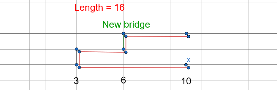
• Eventually, when the new bridge reaches the x-coordinate of the bridge across river 1, the length of the path becomes constant. The path will involve walking left, crossing bridge 1, then walking some amount right, crossing the new bridge across river 2, and walking the rest of the distance right to the destination. As long as the new bridge is between the river 1 bridge and X, the length of the path will remain unchanged.
• Once the new bridge moves past X the length of the path will start increasing by 2km for each kilometer the bridge moves. This is because we need to walk 1km extra to the right to reach the new bridge, and then 1km extra back left to reach the destination.

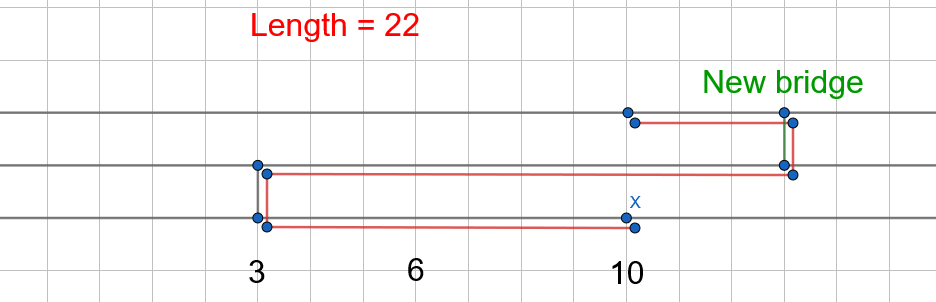
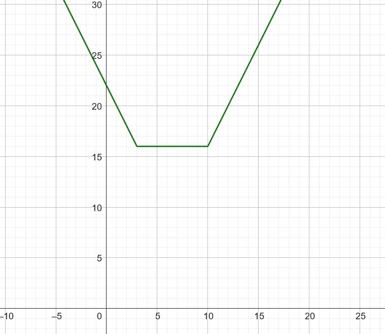
So as we move the new bridge from left to right, the length of the path has a trapezoid-like shape with 3 stages, a decreasing length stage, a constant length stage, followed by an increasing length stage. For example, here is a graph of the path length if the trip has X = 10 and the closest bridge to the left is at X_L = 3.

Taking the minimum length of the closest bridge to the left and closest bridge to the right

We now need to take the minimum of the distance using the closest bridge to the left of X and the distance using the closest bridge to the right of X.

The cost of using the closest bridge to the right of X also has a trapezoid-like shape, and our cost for a particular trip will be the minimum of the two curves at each point. For example, if the trip has X = 10, and the closest bridges to the left and right are at X_L = 3 and X_R = 15, the cost will be the lower part of the two curves:

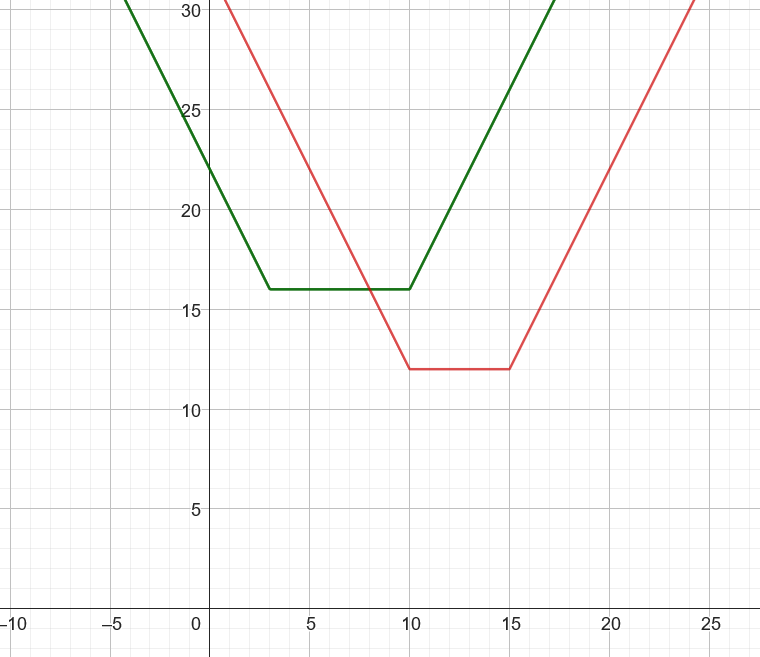
We can see that one of the trapezoids will be lower than the other, depending on which side has the closer bridge to X. Using this understanding of how the cost changes as we move the new bridge from left to right, we can use the same 'sweep' technique from subtask 2. Here is some pseudocode demonstrating this idea:

• Pseudocode

let sum = 0
let rate_of_change = 0
let updates[] be an array storing changes to the rate_of_change

# calculate updates[]
for each trip i (with coordinate X[i]),
    find d_l and d_r = the distances to the closest bridge to the left and right of X[i] respectively
    
    sum += path length if the new bridge is at the leftmost position
    rate_of_change -= 2   # rate of change starts out at -2

    updates[X - d_l] += 2

    if d_r < d_l, then
        # right bridge is closer than left bridge
        updates[X - (d_l - d_r)] -= 2
        updates[X] += 2
    else,
        # left bridge is closer than right bridge
        updates[X] += 2
        updates[X + (d_r - d_l)] -= 2

    updates[X + d_r] += 2

# then same sweepline code as subtask 2

If you're astute, you may notice that the two cases in the code above are actually the same. ;) You will also need to handle the case where there is no bridge to the left or right of a trip's x-coordinate.

One thing to note is that one trapezoid will never be always smaller than the other. For example, even if X = 10 and the closest bridge to the right is also at X_R = 10, the costs look like:

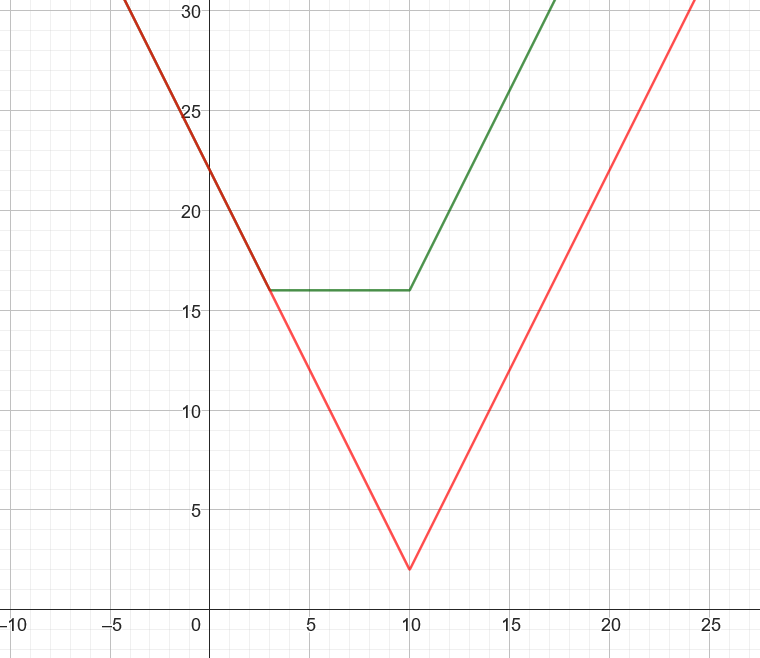
(and this is ignoring the fact that if the closest bridge to the right is at the same x-coordinate as the trip then that bridge will also count as the closest bridge to the left.) Because of this, the above pseudocode will always correctly calculate the cost of each trip.

This allows us to achieve the same time complexity as subtask 2, solving the problem in O(N+T+L) time.

Subtask 4: No special constraints

In the final subtask, there are no special constraints and so we could have existing bridges crossing both rivers and trips that span one or both rivers.

Let's start by assuming the new bridge must be on river 2 like in the previous subtask.

Our analysis of how the length of a trip changes as we move the new bridge from left to right still holds except for one issue. There could be existing bridges on river 2.

What does this change? Well similar to the first 2 subtasks, we can observe that we only care about the current shortest path (that only uses existing bridges) and how that compares to the shortest path using the new bridge.

The shortest path using the new bridge is what we calculated in the previous subtask. It varies depending on the new bridge's position on river 2, but will definitely cross river 1 at either the closest bridge to the left or right of the starting point.

Calculating the current shortest path (the shortest path using only existing bridges)

To calculate the current shortest path, we can use the observation from the previous subtask that the shorest path across both rivers must use the closest bridge to the left or closest bridge to the right of the starting point. The same argument also applies to the endpoint. That is:

Observation: Given a trip ending at coordinate X on Strip 3, it is always optimal to cross river 2 at either:

• the closest bridge to the left of X if one exists (bridge coordinate ≤ X), or
• the closest bridge to the right of X if one exists (bridge coordinate ≥ X)

Proof: The same as above, the argument is symmetrical. QED

Therefore, we just have to precalculate the closest bridge to the left and right (if such bridges exist) on both river 1 and river 2 for each trip, and then try all combinations (of which there are at most 4).

Comparing the current shortest path with the shortest path using the new bridge

We saw that the length of the shortest path using the new bridge, based on the position of the new bridge, can be drawn on a graph as the minimum of two trapezoid-like curves. What does the current shortest path look like?

Well it will have a constant value because it ignores the new bridge's position, so it will just be a flat line. For example, let's take the previous example with a trip at X=10 with closest left and right bridges acrosss river 1 at X_L = 3 and X_R = 15. If there is a bridge across river 2 at x-coordinate 2 and the current shortest path goes through there, then the current shortest path will have length (10-3 + 1 + 3-2 + 1 + 10-2 = 18), so the costs will look like:

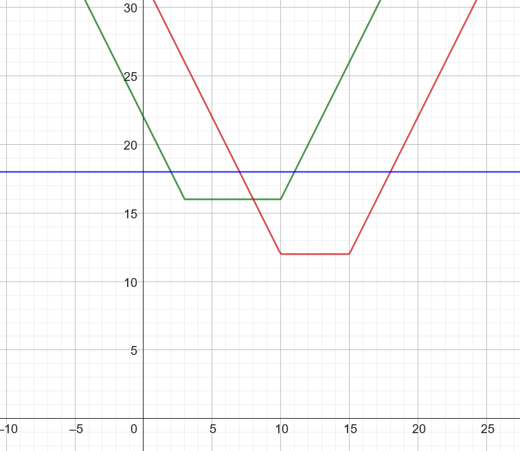
And the final length of the trip, for each new bridge position, will be the minimum of the three curves at each point. We can see that there are 4 stages:

• Initially the current shortest path is the shortest way. (This makes intuitive sense because the new bridge is very far off to the left so it would be very expensive to use it.)
• The path using the closest bridge to the left for river 1 and the new bridge for river 2 is the shortest.
• The path using the closest bridge to the right for river 1 and the new bridge for river 2 is the shortest.
• Then finally, the current shortest path becomes the shortest again.

If we draw out some more cases, we will find that there is one other scenario. For example, if we have the same river 1 bridges, but the current shortest path instead involves a bridge across river 2 at x-coordinate 16, the current shortest path with have length 14, so the costs will look like:

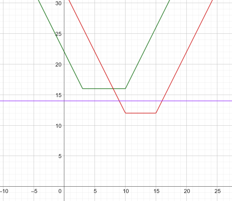
In this case, one of the bridges across river 1 is never optimal to use and we only use either the other bridge with the new bridge, or just take the current shortest path.

Note that the current shortest path cannot be strictly better than both bridges at every point because we have proven that the optimal path must use either the closest left or right bridge.

Putting it all together

So to solve the full case, we have to modify the previous algorithm to handle these two cases where the current shortest path is better than using the new bridge some of the time. Pseudocode demonstrating these ideas (for trips that cross both rivers) might look like:

• Pseudocode

let sum = 0
let rate_of_change = 0
let updates[] be an array storing changes to the rate_of_change

function handle_one_bridge(x1, x2, d, cur_length)
    offset = (cur_length - (2 * d + 2)) / 2
    updates[x1 - offset] -= 2
    updates[x1] += 2
    updates[x2] += 2
    updates[x2 + offset] -= 2

# calculate updates[]
for each trip i across both rivers (with coordinate X[i]),
    find d_l and d_r = the distances to the closest bridge to the left and right of X[i] respectively
    find cur_length = current shortest path length for trip i

    # add current length of trip i to inital sum of trip lengths
    sum += cur_length

    # 2 * d_l + 2 is the shortest possible distance using the left bridge and the new bridge
    if cur_length < 2 * d_l + 2, then
        handle_one_bridge(X, X + d_r, d_r, cur_length)
    else if cur_length < 2 * d_r + 2, then
        handle_one_bridge(X - d_l, X, d_l, cur_length)
    else,
        # both bridges will be optimal (or equally optimal) at various times
        # this case is similar to subtask 3

        left_offset = (cur_length - (2 * d_l + 2)) / 2
        updates[X - d_l - left_offset] -= 2

        updates[X - d_l] += 2
        
        # this code was split into two cases that actually did the same thing before
        updates[X] += 2
        updates[X + d_r - d_l] -= 2
        
        updates[X + d_r] += 2

        right_offset = (cur_length - (2 * d_r + 2)) / 2
        updates[X + d_r + right_offset] -= 2

# perform sweep using sum, rate_of_change and updates[] as in previous subtasks

What remains is:

• to handle trips that cross one river (if a trip is on the same side as the new bridge it is similar to subtasks 1 and 2, otherwise it adds a constant cost no matter where the new bridge is), and
• to handle whether the new bridge is on river 1 or river 2. One possible way to implement this is to have a function that solves the problem assuming the bridge is on a specific river. Then you can call this function once, swap the bridges and one-river trips between the rivers, then call the function again.

This was a challenging problem to solve and especially a challenging problem to implement, particularly for the AIO level. Good luck!

Click here to go back.